
Fastest Doesn’t Always Mean Best: Optimising an Edge AI Pipeline on Rubik Pi 3

Written by
Karol Adamiak
Software Engineer

Executive Summary (TL:DR)
- Our starting point (previous article): moving AI compute from a CPU to a dedicated accelerator (NPU) required a one-line code change and delivered ~8.7× higher FPS, ~11× lower energy per frame, and a −16 °C temperature drop compared to a Raspberry Pi 5 CPU. But that’s only a prototype: the NPU crunches numbers in a flash, yet there’s still room to push for better results.
- This article’s thesis is that once you’ve chosen an accelerator, you can further improve performance through software architecture. You need to make full use of the available hardware and parallelise the work around the NPU. To do that deliberately, you must measure FPS, latency, CPU & RAM usage, chip temperature, and power draw.
- Three approaches were tested, each with a different trade-off: a multithreaded Python pipeline (2.1× faster: 36→75 FPS), a full rewrite in C++ (a speed ceiling of ~94 FPS), and a fully hardware-driven GStreamer pipeline (slower at ~81 FPS, but using the least CPU and the least energy per frame).
Bottom line
- Fastest ≠ best. Those are short-sprint numbers, and under sustained load, Python and C++ climb to ~91 and ~81 °C (throttling), while the full GStreamer pipeline holds steady at ~64 °C and ~4.8 W.
- C++ wins the sprint; putting the work fully on hardware wins the race.
From prototype to product
In the previous article, we asked where to run the AI model: on a general-purpose CPU or on a dedicated accelerator (NPU, a chip built specifically for neural networks).
The answer was clear-cut: the same two-stage PPE (personal protective equipment: helmet, vest) detection system on the Rubik Pi 3’s NPU ran ~8.7× faster, used ~11× less energy per frame, and ran ~16 °C cooler than on a Raspberry Pi 5 CPU. Enabling the NPU was practically a one-line code change.
But that’s only a working prototype, not a product. The telltale symptom: the NPU alone analyses one frame in a fraction of a second, yet the whole system still doesn’t reach the pace the accelerator is capable of.
The reason is mundane: the NPU waits on the CPU to read a frame from the video, resize it, prepare data for the model, crop people out, and post-process the results. In a naive implementation, all of this happens one step at a time, and the accelerator sits idle most of the time.
What Edge AI “optimisation” really means
Once you’ve chosen the accelerator, further gains don’t come from “computing AI faster”; that’s fixed by the hardware and the model. They come from how you organise the work around the AI. Optimisation boils down to two levers:
- Offloading the CPU: moving as much work as possible from the general-purpose processor onto specialised blocks in the chip (NPU, GPU, hardware video decoder), so the CPU is neither a bottleneck nor a disproportionate power draw.
- Parallel work: arranging the successive steps (video read, pre-processing, AI inference, post-processing) so they happen at the same time instead of waiting on each other. Then the NPU gets a steady stream of work.
Important: there’s no single “best” method. Every optimisation step costs something: in code complexity, CPU usage, memory, sometimes single-frame latency. The right approach depends on your resource budget: how much CPU and RAM you have, whether the device runs on battery, whether it’s passively cooled and running 24/7, and whether image analysis is its only job or one of several.
You can’t optimise what you don’t measure
Each of the levers above is a trade-off, and a trade-off can’t be judged “by eye”. So, before we start speeding things up, we need to establish what we measure and how. This is the foundation of the whole article: every number below comes from a repeatable measurement on the same device and the same video material.
| Parameter | What it tells you | How it’s measured |
|---|---|---|
| Throughput (FPS) | how many frames per second the system actually processes | frame count / wall-clock time; warm-up excluded from the measurement |
| Latency | time for a single frame to travel from input to result | a timestamp on every frame; matters for how fast a safety system reacts |
| CPU / memory usage | how much CPU and RAM a variant “consumes” | background sampling during the run |
| Chip temperature | whether the chip is heating up and approaching throttling (the forced slowdown that kicks in when it overheats) | on-chip temperature sensors |
| Power and energy/frame | real draw from the wall outlet; the energy cost of a single frame | external ChargerLAB Power-Z meter, sliced by timestamps |
Two things in the methodology are worth calling out.
- We measure power in hardware, with an external meter on the power cable, not “in software”, because a reading taken from the device itself is incomplete and loads the measurement.
- Energy per frame (power × time / frame count) is often a more important metric than FPS alone: it shows what a model’s “decision” really costs, which determines battery life and whether the device can be passively cooled.
Step I: multithreading in Python, feeding the NPU
The first and cheapest step doesn’t even require changing the programming language. It’s enough to notice that our loop does everything one step at a time:
read a frame → model 1 (where’s the person) → crop the person out → model 2 (do they have a helmet and vest) → save the result
While the NPU works, the CPU waits. While the CPU works, the NPU waits. Nobody does two things at once.
You can see this when you break a single frame down into stages. Six steps line up in sequence, with the engines lighting up alternately: prep and post-processing on the CPU, and inference on the NPU.
The CPU stages add up to ~9.7 ms, the NPU stages to ~9.5 ms, but since they never run at the same time, the frame takes their sum (~19.1 ms), and each engine sits underused for half the time. This is exactly where the idea of using concurrent processing comes from.
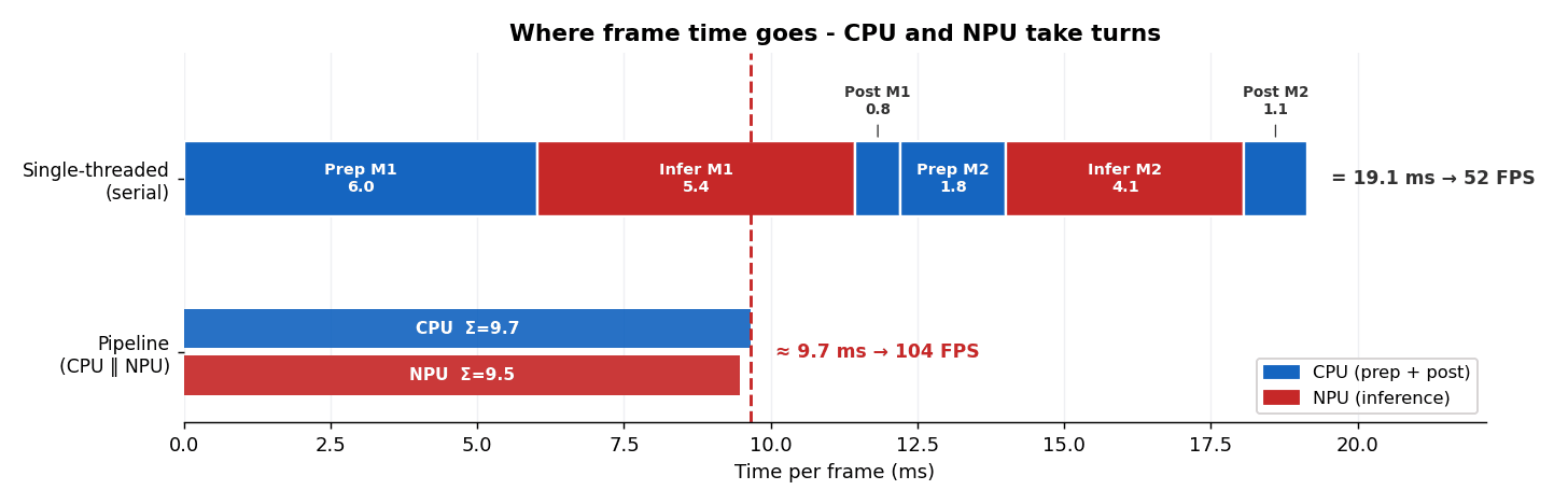
A single frame in single-threaded mode, broken into six stages (top bar): CPU stages (prep/post-processing) and NPU stages (inference) run alternately; while one engine works, the other waits. If the two tracks were overlaid (bottom bars), the frame time would be set by the slower of the two engines, not their sum; that’s the pipeline’s theoretical ceiling. These times cover pure compute; the “wall” FPS achieved in the table is lower due to decode and loop overhead, but the same ~2× headroom remains. Times averaged over the entire run.
The fix is concurrent processing. Instead of one worker doing everything, we spin up five running in a cascade, each handling a different stage at the same moment.
read → model 1 → crop → model 2 → write
While model 1 is analysing frame 10, the reader is already fetching frame 11, and the writer is finishing frame 9. The NPU gets a steady stream of work.
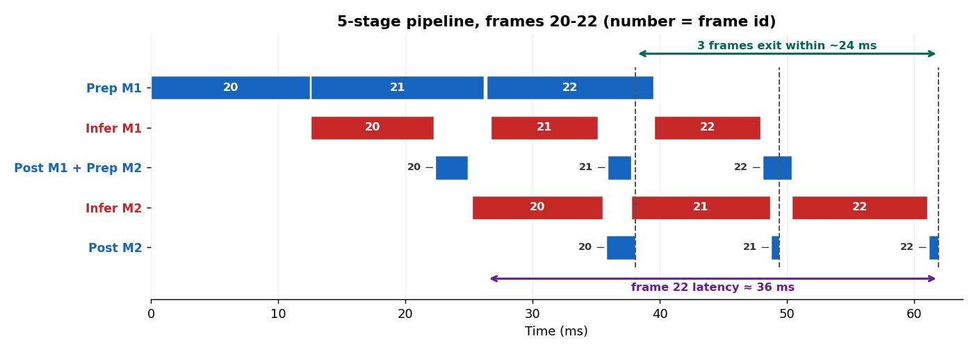
Three frames from steady state (once every worker already has something queued, frames 20–22), using real timestamps from an NPU run. The number in each box is the frame number; NPU stages are red, CPU stages blue.
Notice the offset: while the reader is on frame 22, Model 1 is still working on frame 21, and Model 2 is finishing frame 20: several frames in flight across different stages at once. That’s the time single-threaded mode left on the table.
The two arrows show the heart of the trade-off: three frames leave the pipeline within ~24 ms of each other; that’s throughput. But a single frame may spend ~36 ms in the pipeline, compared to ~19 ms in single-threaded mode: that’s latency.
The pipeline buys throughput at the cost of latency. Two subtleties are visible directly: the pace is set by the longest stage (blue reader), not the sum of all of them; and the red Model 1 and Model 2 blocks are longer than pure inference, because both models share one NPU and wait on each other (~1.4–1.9× longer in the pipeline than measured standalone).
Parallelising isn’t free. When we measure the average time for each stage separately (once single-threaded, once in the pipeline), the same stage takes longer in the pipeline for two reasons.
- CPU stages (prep, post-processing) swell because five threads compete for one Python interpreter (the GIL) and for cores;
- NPU stages (inference) swell because both models share one Hexagon and queue behind each other. The per-frame total grows by ~50%, yet throughput still doubles, because the stages overlap in time.
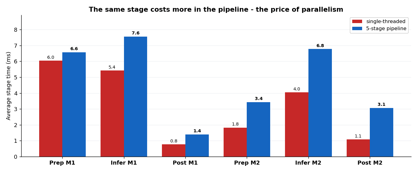
Average time of each of the six stages: single-threaded (red) vs pipeline (blue), the same work on the same material. Every stage takes longer in the pipeline: CPU stages (prep and post-processing) due to the GIL and thread contention; NPU stages (Model 1 and Model 2 inference) due to sharing one Hexagon. The per-frame total grows by ~50%, but overlapping the stages (Gantt above) still yields 2× higher throughput: a price well worth paying. Times averaged over the entire run.
| Parameter | Sequential (1 worker) | Pipeline (5 workers) | Change |
|---|---|---|---|
| Throughput | 36 FPS | 75 FPS | 2.1× faster |
| Single-frame latency (average) | 19.1 ms | 25.0 ms | slightly higher |
| CPU usage (mean/max) | 38 / 46 % | 60 / 71 % | the price of speed |
| RAM | 387 MB | 416 MB | ≈ the same |
| Chip temperature (mean / max) | 49 / 51 °C | 61 / 64 °C | warmer |
| Power draw | 3.98 W | 6.39 W | more |
| Energy per frame | 110 mJ | 86 mJ | 1.3× less |
The effect is clear: more than double the frames per second. But there’s also a visible price: the CPU works harder (from 38% to 60%), the chip runs hotter (49 → 61 °C, and this still isn’t a long-term test, just a short run over 1,500 frames), and instantaneous power draw rises (from 3.98 to 6.39 W), because now several things are genuinely happening at once.
What matters most, though, is energy per frame: how much power one system “decision” costs. Despite the higher instantaneous power, the pipeline produces so many more frames that a single frame costs 86 millijoules instead of 110: the chip is more efficient per frame, even though it runs hotter.
Single-frame latency does creep up a little (19 → 25 ms), because a frame now “travels” through five workers. For a system that just needs to keep up, that’s a great trade-off. For one that needs to react in a split second, it’s worth keeping in mind.
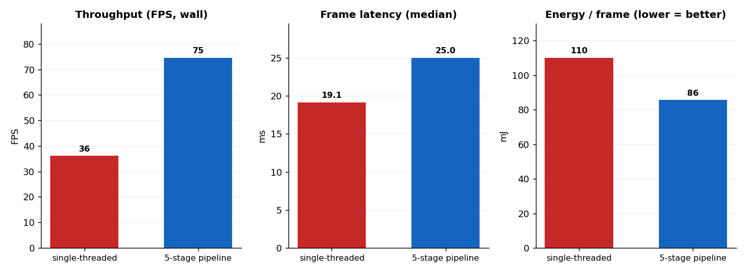
Moving from “one step at a time” processing to a 5-stage pipeline: over 2× more frames per second and ~⅓ lower energy per frame, at the cost of slightly higher single-frame latency.
Step II: the language tax, rewriting in C++
Now that the CPU is loaded, the next question is: how much does Python itself cost us? We rewrite the same 5-stage pipeline in C++ (the same AI library, the same NPU, only the language changes) and compare it across two video-decode variants:
- software (H.264 decoding on the CPU, the same way Python does it) and
- hardware (decoding on a dedicated video block in the SoC; the CPU only receives finished frames).
The AI in both variants runs on the same NPU; the only difference is who unpacks the video.
| Variant | FPS | model 1 / 2 time (ms) | decode (ms) | CPU % | RAM (MB) | Power | Energy/fr. |
|---|---|---|---|---|---|---|---|
| Python | 75 | 7.7 / 7.4 | 6.9 | 61 | 411 | 6.84 W | 92 mJ |
| C++ (sw) | 40 | 5.8 / 5.5 | 23.5 | 22 | 366 | 4.99 W | 126 mJ |
| C++ (hw) | 94 | 9.2 / 10.3 | 7.3 | 39 | 592 | 6.09 W | 65 mJ |
The most important thing is what is not obvious at first glance: the AI itself costs the same regardless of the programming language – in every variant, the same NPU computes it. Measured without contention, in the single-threaded mode, that is ~9.5 ms of NPU work per frame (5.4 ms for model 1 + 4.1 ms for model 2).
The model times in the table are higher, and they grow with throughput (5.8 / 5.5 ms at 40 FPS; 7.7 / 7.4 at 74; 9.2 / 10.3 at 94). This is not a contradiction but a consequence of both models sharing one NPU: the measured inference time also covers waiting in the queue, not just computing. The conclusion is unchanged: at this stage the language cannot be “made faster”; the difference comes from the code around the AI and from how the video is read from the file.
This gives a surprising result: Python (75 FPS) beats C++ with a software video decoder (40 FPS). The reason is, again, mundane: Python’s OpenCV library uses a fast, multi-core decoder, while our baseline C++ variant uses a slower, single-core one. So Python’s cost shows up not in speed, but in CPU load and current draw: C++ does the same job while using 22% CPU instead of 61%. Only C++ with the hardware decoder reaches ~94 FPS at the lowest energy per frame (65 mJ): the practical speed ceiling for this pipeline.
There’s also a non-obvious difference in memory. C++ with the software decoder leaves the smallest footprint: ~366 MB, less than Python (~411 MB). But C++ with the hardware decoder takes ~592 MB: the hardware path loads the entire Qualcomm GPU/EGL stack (the Adreno driver), which the software decoder never touches. In other words, the hardware decoder buys FPS but pays for it in memory; Python (software decoder via OpenCV) never pulls that stack in.
Step III: everything on hardware, GStreamer
The last step is handing off the entire job to hardware. We build a pipeline in GStreamer (Qualcomm’s ready-made multimedia pipeline “construction kit”) where every stage runs on a specialised block of the chip:
hardware video decoder → both AI networks on the NPU → cropping and drawing boxes on the GPU → hardware video encoder
The general-purpose CPU barely touches individual frames; it just keeps the whole data flow through the pipeline running smoothly.
| Parameter | GStreamer cascade (person + PPE, full HW) |
|---|---|
| FPS | 81 |
| CPU | 27% |
| RAM peak | 377 MB |
| Power (mean, from the long run) | ~4.8 W |
| Energy / frame | ~59 mJ |
In terms of raw speed, GStreamer (~81 FPS) is slightly slower than C++ (~94 FPS). That comes down to how each is built. A hand-written C++ pipeline overlaps tasks more intelligently, while GStreamer’s ready-made, “assembled from blocks” graph adds overhead passing frames between successive blocks.
In exchange, though, we get something more valuable than raw frames.
GStreamer uses ~⅔ the CPU compared to C++ (27% vs 39%) and uses the least memory: ~377 MB, less than Python (411 MB) and less than C++ with the hardware decoder (592 MB, since it loads the GPU/EGL Adreno stack).
That flips the narrative from “GStreamer is slower” to “GStreamer leaves the most resources available for the rest of the system, at the lowest energy per frame”.
Not a black box: detections as a stream
Handing the work to hardware doesn’t mean losing access to the results. Detections can be “tapped” straight out of the GStreamer pipeline and exposed as a simple text stream (JSON), one line per frame, ready to be read by a separate alert application (“a person appeared without a helmet or vest”):
{"frame":137, "pts_ns":5480000000, "persons":[

{"id":256, "bbox":[889,587,134,402], "helmet":true, "vest":false, "ppe_ok":false}],

"alert":true}
Crucially, the system already knows which vest belongs to which person: every helmet or vest detection is tied to a specific individual, so there’s no need to guess it from box positions.
The same pipeline that’s the coolest and lightest also hands off ready-made, structured input for safety logic.
The big showdown and the endurance test
Let’s bring it all together in one table. To keep the comparison fair, every number below comes from one single, continuous long-term test: the same conditions, the same material, the same power-measurement session.
| Parameter | Python (pipeline) | C++ (GStreamer decode) | GStreamer (full HW) |
|---|---|---|---|
| FPS (sustained) | ~73 | ~89 | ~81 |
| CPU (mean) | ~62 % | ~40 % | ~27 % |
| RAM peak | ~411 MB | ~592 MB | ~377 MB |
| Power (mean) | 7.52 W | 6.54 W | 4.79 W |
| Energy / frame | 103 mJ | 74 mJ | 59 mJ |
| Steady-state temp (max) | 91 (92) °C | 81 (82) °C | 64 (65) °C |
The endurance test (long-run)
Peak FPS is a sprint result. The more interesting production question is: what happens when the pipeline runs non-stop? So each variant was held under sustained load, with SoC temperature, clock throttling, CPU, and power draw recorded over time.
Hypothesis:
- C++ is the fastest but puts the CPU under heavy load: under sustained load, it heats up above the throttling threshold, and power draw stays high.
- The full GStreamer pipeline gives up peak FPS, but holds a flat, cool, stable line: that’s the one you leave running permanently.
The measurement confirms it.
- The Python and C++ pipelines reach ~91 and ~81 °C at steady state, right at the edge of throttling, drawing 7.5 and 6.5 W, respectively; clock speed starts to drop.
- The full GStreamer pipeline holds a flat ~64 °C at 4.8 W and 27% CPU: over 20 °C cooler and significantly less power.
- The energy/frame gap is smaller (59 vs 74 vs 103 mJ), because C++ makes up for it with higher FPS.
- But it’s thermals and power, not energy, that decide what you leave running 24/7 in a passively cooled enclosure.
- Measurement fairness: every variant started from the same cooled-down baseline (before each run, the SoC was idle for a long period and allowed to drop to <50 °C), so the curves are directly comparable and not skewed by residual heat from the previous run.
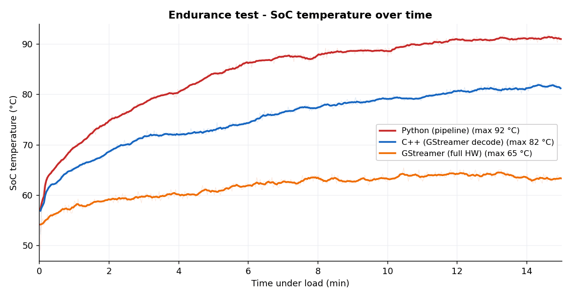
SoC temperature under sustained load. Python and C++ climb to ~91 and ~81 °C (the edge of throttling; clock speed starts dropping), while the full GStreamer pipeline holds a flat ~64 °C for the whole run.
Every variant started from a cooled-down chip (<50 °C); each run waited until the temperature returned to the shared thermal baseline first, so the curves are comparable.
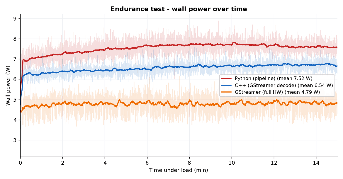
Power draw from the wall outlet (ChargerLAB Power-Z). GStreamer holds ~4.8 W, much less than Python (~7.5 W) and C++ (~6.5 W).
Conclusions
Edge AI optimisation doesn’t end with picking an accelerator: that’s where it starts.
Three steps (concurrent processing → migrating to C++ → fully offloading to hardware via GStreamer) show that every gain has a price, and the right choice depends on what the production requirements are:
- C++: when the device’s only job is image analysis as fast as possible.
- The full GStreamer pipeline: when the device also does something else, has a RAM/energy budget, or runs passively cooled 24/7.
- Multithreaded Python: when deployment and maintenance speed matter, and there aren’t very tight compute constraints.
The key takeaway: you can’t make any of these choices without measuring. Fastest doesn’t always mean best for every industrial project.
Consult Red designs and optimises Edge AI systems from model to production device: accelerator selection, pipeline architecture, power and thermal budgeting, deployment on target hardware. If you’re facing a similar problems, get in touch.
Appendix: test environment
For reproducibility, here’s the full hardware and software specification on which every number in this article was collected (Rubik Pi 3, built and run on the device itself).
| Layer | Details |
|---|---|
| Device / SoC | Rubik Pi 3, Qualcomm QCS6490; 8 aarch64 cores: 4× Cortex-A78 (≤ 2.71 GHz) + 4× Cortex-A55 (≤ 1.96 GHz); Hexagon NPU (via the QNN HTP delegate) |
| OS | Ubuntu 24.04.4 LTS · kernel 6.8.0-1079-qcom (aarch64) |
| Toolchain (built on-device) | gcc / g++ 13.3.0 · CMake 3.28.3 · GNU Make 4.3 · ld (binutils) 2.42 · glibc 2.39 · C++17 |
| NPU delegate (shared) | QAIRT / QNN SDK 2.44.0 (qnn_backend_api 2.18.0) · libQnnTFLiteDelegate.so + HTP backend |
| Video | GStreamer 1.24.2 |
The AI core in both implementations is the same LiteRT runtime (Google AI Edge) on the same NPU; only the delivery method and the libraries around it differ:
| Component | Python | C++ |
|---|---|---|
| AI runtime | ai-edge-litert 2.1.6 (pip) | LiteRT from source (google-ai-edge/LiteRT, commit 11ac389) |
| Language / version | Python 3.12.3 | C++17 (gcc 13.3.0) |
| OpenCV | 4.10.0.84 (opencv-python-headless) | 4.6.0 (system) |
| Other | numpy 2.5.1 | TensorFlow v2.21.0-rc0: build-time headers only (schema/TSL/XLA),not the inference runtime |
If you are interested in reproducing these results, the full benchmark code, covering the LiteRT inference pipeline, the thread-scaling tests, and thermal logging, is available on our GitHub. Power was measured externally with a USB power meter (ChargerLAB Power-Z), so it isn’t part of the code.
Some images on this page are AI-generated and used for illustrative purposes.
Related Insights

Articles
Generative AI at the Edge: What’s Possible in 2026
Advances in NPU capabilities and quantization have enabled more sophisticated AI models running locally for low-latency, lower-cost and secure applications.
Articles
The Joy of PoCs
Why a small and early proof of concept (PoC) can save you much, much more in the long run.

Videos
Simply Explained: Why Your Router Should Be Doing the AI in the Connected Home
Watch our CTO, Rahul Mehra, unpack the full case for anchoring edge AI in the broadband router.